---

A digital image is composed with a countable number of picture elements which are also known as pixels. The digital image capturing devices such as smart phones and digital cameras capture the light signals from objects and breaks up them into millions of picture elements. But during this process the capturing devices tend to introduce various types of noises to the images. These noises can be occurred due to various reasons such as heat, electricity, and the amount of sensor illumination levels. As of these noises in images the quality of the image is reduced. However, there are some basic to advance algorithms in digital image processing to reduce these types of noises from images and enhance the quality of images. These algorithms are called Image smoothing algorithms. In this article, I am going to explain some of those algorithms.

What is Noise?

Noise can be found in any form of signals. It is unexpected interference that reduce the quality of the signal. In digital images, the noise is unexpected color variations in an image that reduce the quality of the image. There are various types of noises available in the images. But in this article, I am going to talk about the impulse noises.

What are Impulse noises?

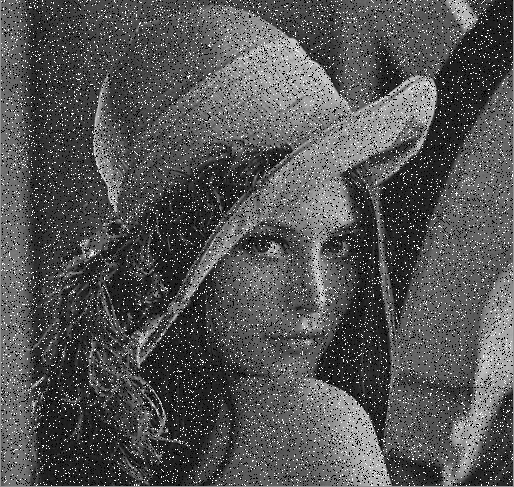
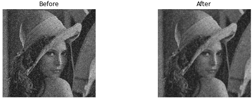
The impulse images are usually occurred due to a failure in the image capturing device. The impulse noises replace some of the pixel values of the original images. There are two main types of impulse noises. First one is the salt-and-pepper noise, which can have only two values either 0 or 255. The second one is random-values impulse noise. Which can take any of the whole values between 0 to 255. In this article I am going to take one example for salt-and-pepper noise and show how different types of noise reduction algorithm so-called image smoothing algorithms work. The image below, lenna image, is the example image that I am going to use throughout this article.

Types of Smoothing Algorithms

There are various types of image smoothing algorithms. This article covers the following smoothing algorithms.

1. Mode Filter
2. Median Filter
3. Mean Filter
4. Gaussian Filter

Kernel

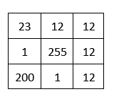
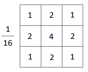
In image processing, a kernel, convolutional matrix or mask is a small matrix of size 3 * 3, 5 * 5 or etc. Which is can be used to perform operations such as filtering. Following is a sample kernel.

Mode Filter

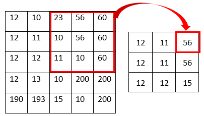
The mode filter is one of a simplest image smoothing algorithms. In this algorithm each pixel of the original image is going to be replaced by the mode value of its neighboring pixels. The neighboring pixels can be determined by considering the kernel. Following example shows how the mode filter works.

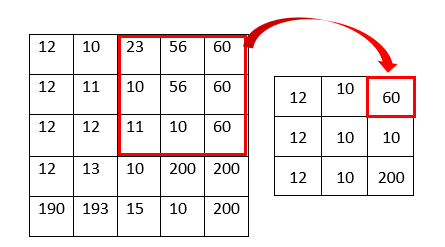
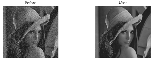
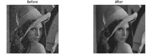
As shown in the above figure the pixel value is the mode value of the kernel. For example, the top right pixel value of the resulting image becomes 60 because the mode of the kernel is 60 (23, 56, 60, 10, 56, 60, 11, 10, 60). The image below shows before and after result of the example image.

Median Filter

The median filter is also one of the simplest image smoothing algorithms. In this algorithm, each pixel of the original image is going to be replaced by the median value of its neighboring pixels. The neighboring pixels can be determined by considering the kernel. Following example shows how the median filter works.

As shown in the above figure, the pixel value is the median value of the kernel. For example, the top right pixel value of the resulting image becomes 56 because the median of the kernel is 56 (10, 10, 11, 23, 56, 56, 60, 60, 60). The image below shows before and after result of the example image.

Mean Filter

The mean filter is also known as averaging filter as it takes the average values of the neighboring pixels. In this algorithm, each pixel of the original image is going to be replaced by the mean value of its neighboring pixels. The neighboring pixels can be determined by considering the kernel. Following example shows how the mean filter works.

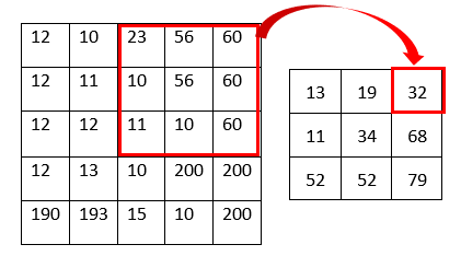
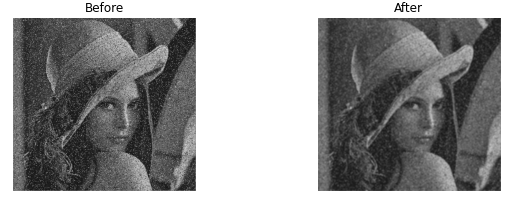
As shown in the above figure, the pixel value is the mean value of the kernel. For example, the top right pixel value of the resulting image becomes 32 because the mean of the kernel is 32 ((10 + 10 + 11 + 23 + 56 + 56 + 60 + 60 + 60)/9 = 32). The image below shows before and after result of the example image.

Gaussian Filter

The gaussian filter is almost same as the mean filter but in the mean filter all the neighboring pixels have the same weight regardless of the distance from the center pixel. In this mean filter, the pixels that are far away from the center pixel contribute same as the pixel that are closest to the center pixel. This may cause error like under and over calculation. So, in the gaussian filter the neighboring pixels are assigned a weight based on the distance from the center pixel. The kernel for the gaussian filter can be calculated with the help of 2D gaussian function. Following is the 2D gaussian function.

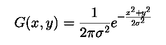
In the above equation x and y are the coordinates of the pixel and sigma can be varied from 1 to any number. Following is the sample 3 * 3 kernel for gaussian filter when sigma is 1.

Following image shows how to calculate the resulting image using gaussian filter.

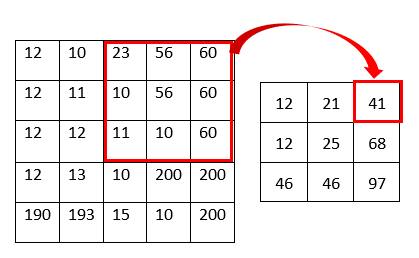
As shown in the above figure, the pixel value is the gaussian average value of the kernel. For example, the top right pixel value of the resulting image becomes 41 because the gaussian average of the kernel is 41 ((23 * 1 + 56 * 2 + 60 * 1 + 10 * 2 + 56 * 4 + 60 * 2 + 11 * 1 + 10 * 2 + 60 * 1)/16 = 41). The image below shows before and after result of the example image.

Summary

Due to some issues in image capturing devices and environments, the digital images come up with some noises which can reduce the quality of the image. In this article, I discussed Impulse Noise and its most common version of salt-and-pepper noise. After that I discussed four main types of image filtering algorithms that can be used to reduce the salt-and-pepper noise. They are Mode Filter, Median Filter, Mean Filter and Gaussian Filter.

References

https://docs.opencv.org/4.x/d4/d13/tutorial_py_filtering.html